Example: Light Curve Generation

This page shows how to combine lightcurve-strategies with jaxoplanet.starry.light_curves.light_curve to generate and test transit light curves end-to-end.

Creating a SurfaceSystem

Use surface_systems() with st.just() to pin specific parameters while letting Hypothesis control the rest. Here we create a Sun-like star with quadratic limb darkening and a single transiting planet:

from hypothesis import strategies as st
from lightcurve_strategies import (
    centrals,
    bodies,
    surfaces,
    surface_systems,
)

# Fixed central star: 1 M_sun, 1 R_sun, quadratic limb darkening
star = centrals(mass=st.just(1.0), radius=st.just(1.0))
star_surface = surfaces(u=st.just((0.1, 0.3)))

# Fixed planet: 3-day period, radius ratio 0.1
planet = bodies(period=st.just(3.0), radius=st.just(0.1))
planet_surface = surfaces()

# Combine into a SurfaceSystem strategy with exactly 1 body
system_strategy = surface_systems(
    central=star,
    central_surface=star_surface,
    body=st.tuples(planet, planet_surface),
    min_bodies=1,
    max_bodies=1,
)

Computing the light curve

Once you have a SurfaceSystem, pass it to jaxoplanet.starry.light_curves.light_curve along with a time array:

import jax.numpy as jnp
from hypothesis import given, settings
from jaxoplanet.starry.light_curves import light_curve

@given(system=system_strategy)
@settings(max_examples=1)
def test_compute_light_curve(system):
    # Evaluate around mid-transit
    time = jnp.linspace(-0.2, 0.2, 200)
    # light_curve returns shape (N, n_bodies); column 0 is the star
    flux = light_curve(system, order=10)(time)[:, 0]

    print(f"flux min = {flux.min():.6f}")
    print(f"flux max = {flux.max():.6f}")
    assert flux.shape == (200,)

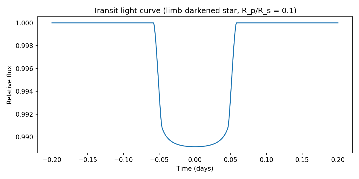
Transit light curve

The plot below is generated during the docs build. It constructs a SurfaceSystem with fixed parameters and evaluates the light curve around mid-transit:

import jax.numpy as jnp
import matplotlib.pyplot as plt
from hypothesis import strategies as st
from lightcurve_strategies import bodies, centrals, surfaces, surface_systems
from jaxoplanet.starry.light_curves import light_curve

# Build a deterministic SurfaceSystem (no randomness needed for the plot)
star = centrals(mass=st.just(1.0), radius=st.just(1.0))
star_surface = surfaces(u=st.just((0.1, 0.3)))
planet = bodies(
    period=st.just(3.0),
    radius=st.just(0.1),
    time_transit=st.just(0.0),
    impact_param=st.just(0.3),
)
planet_surface = surfaces()
system_strategy = surface_systems(
    central=star,
    central_surface=star_surface,
    body=st.tuples(planet, planet_surface),
    min_bodies=1,
    max_bodies=1,
)

system = system_strategy.example()
time = jnp.linspace(-0.2, 0.2, 500)
# light_curve returns shape (N, n_bodies); column 0 is the star
flux = light_curve(system, order=10)(time)[:, 0]

fig, ax = plt.subplots(figsize=(8, 4))
ax.plot(time, flux, color="tab:blue", linewidth=1.5)
ax.set_xlabel("Time (days)")
ax.set_ylabel("Relative flux")
ax.set_title("Transit light curve (limb-darkened star, R_p/R_s = 0.1)")
fig.tight_layout()

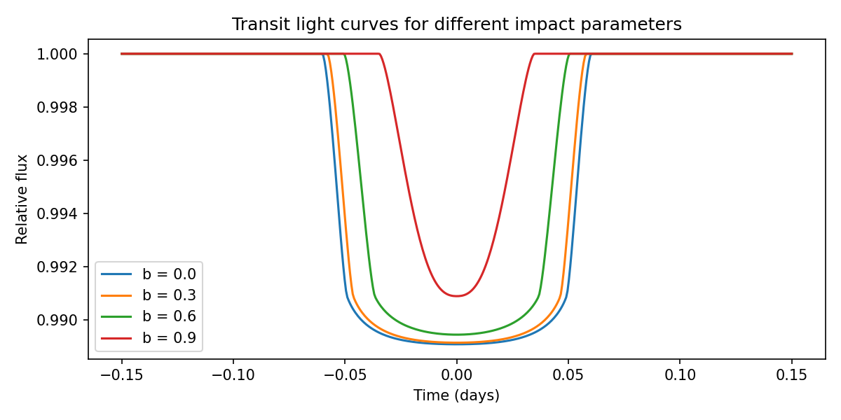
Impact parameter comparison

Varying the impact parameter changes the transit depth and shape. This plot overlays light curves for several impact parameters:

import jax.numpy as jnp
import matplotlib.pyplot as plt
from hypothesis import strategies as st
from lightcurve_strategies import bodies, centrals, surfaces, surface_systems
from jaxoplanet.starry.light_curves import light_curve

star = centrals(mass=st.just(1.0), radius=st.just(1.0))
star_surface = surfaces(u=st.just((0.1, 0.3)))

time = jnp.linspace(-0.15, 0.15, 500)

fig, ax = plt.subplots(figsize=(8, 4))
for b_val in [0.0, 0.3, 0.6, 0.9]:
    planet = bodies(
        period=st.just(3.0),
        radius=st.just(0.1),
        time_transit=st.just(0.0),
        impact_param=st.just(b_val),
    )
    system = surface_systems(
        central=star,
        central_surface=star_surface,
        body=st.tuples(planet, surfaces()),
        min_bodies=1,
        max_bodies=1,
    ).example()
    flux = light_curve(system, order=10)(time)[:, 0]
    ax.plot(time, flux, linewidth=1.5, label=f"b = {b_val}")

ax.set_xlabel("Time (days)")
ax.set_ylabel("Relative flux")
ax.set_title("Transit light curves for different impact parameters")
ax.legend()
fig.tight_layout()

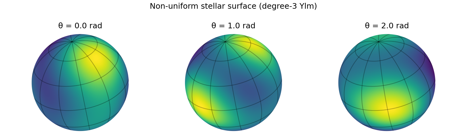
Non-uniform stellar surface

Real stars are not featureless — spots, faculae, and other surface inhomogeneities modulate the transit light curve. In jaxoplanet, these features are encoded as spherical harmonic maps using Ylm. The surfaces() strategy accepts a y parameter so you can pass a pre-built map:

import numpy as np
from hypothesis import strategies as st
from jaxoplanet.starry.ylm import Ylm
from lightcurve_strategies import surfaces

np.random.seed(42)
y = Ylm.from_dense([1.00, *np.random.normal(0.0, 2e-2, size=15)])
spotted_surface = surfaces(y=st.just(y), inc=st.just(1.0),
                           obl=st.just(0.2), period=st.just(27.0),
                           u=st.just((0.1, 0.1)))

Surface map

The plot below shows the spherical harmonic surface map used in this example, rendered with show_surface:

import numpy as np
import matplotlib.pyplot as plt
from jaxoplanet.starry.ylm import Ylm
from jaxoplanet.starry.surface import Surface
from jaxoplanet.starry.visualization import show_surface

np.random.seed(42)
y = Ylm.from_dense([1.00, *np.random.normal(0.0, 2e-2, size=15)])
surface = Surface(inc=1.0, obl=0.2, period=27.0, u=(0.1, 0.1), y=y)

fig, axes = plt.subplots(1, 3, figsize=(10, 3))
for ax, theta in zip(axes, [0.0, 1.0, 2.0]):
    plt.sca(ax)
    show_surface(surface, theta=theta, ax=ax)
    ax.set_title(f"θ = {theta:.1f} rad")
fig.suptitle("Non-uniform stellar surface (degree-3 Ylm)")
fig.tight_layout()

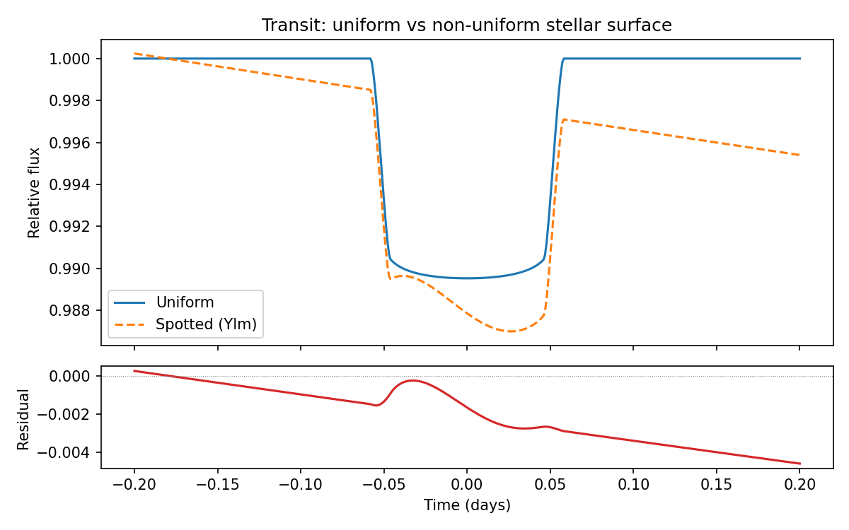
Uniform vs non-uniform transit

Comparing a uniform and a spotted star with the same orbital parameters highlights the residuals introduced by the surface map. This plot demonstrates the y parameter of surfaces() in action:

import jax.numpy as jnp
import numpy as np
import matplotlib.pyplot as plt
from hypothesis import strategies as st
from jaxoplanet.starry.ylm import Ylm
from jaxoplanet.starry.light_curves import light_curve
from lightcurve_strategies import bodies, centrals, surfaces, surface_systems

# Shared orbital parameters
star = centrals(mass=st.just(1.0), radius=st.just(1.0))
planet = bodies(
    period=st.just(3.0),
    radius=st.just(0.1),
    time_transit=st.just(0.0),
    impact_param=st.just(0.3),
)

# Uniform star
uniform_system = surface_systems(
    central=star,
    central_surface=surfaces(u=st.just((0.1, 0.1))),
    body=st.tuples(planet, surfaces()),
    min_bodies=1, max_bodies=1,
).example()

# Non-uniform star
np.random.seed(42)
y = Ylm.from_dense([1.00, *np.random.normal(0.0, 2e-2, size=15)])
spotted_system = surface_systems(
    central=star,
    central_surface=surfaces(
        y=st.just(y), inc=st.just(1.0), obl=st.just(0.2),
        period=st.just(27.0), u=st.just((0.1, 0.1)),
    ),
    body=st.tuples(planet, surfaces()),
    min_bodies=1, max_bodies=1,
).example()

time = jnp.linspace(-0.2, 0.2, 500)
flux_uniform = light_curve(uniform_system, order=10)(time)[:, 0]
flux_spotted = light_curve(spotted_system, order=10)(time)[:, 0]

fig, (ax1, ax2) = plt.subplots(2, 1, figsize=(8, 5), sharex=True,
                                gridspec_kw={"height_ratios": [3, 1]})
ax1.plot(time, flux_uniform, label="Uniform", linewidth=1.5)
ax1.plot(time, flux_spotted, label="Spotted (Ylm)", linewidth=1.5,
         linestyle="--")
ax1.set_ylabel("Relative flux")
ax1.set_title("Transit: uniform vs non-uniform stellar surface")
ax1.legend()

ax2.plot(time, flux_spotted - flux_uniform, color="tab:red", linewidth=1.5)
ax2.set_xlabel("Time (days)")
ax2.set_ylabel("Residual")
ax2.axhline(0, color="gray", linewidth=0.5, linestyle=":")
fig.tight_layout()

Property-based test

The real power of lightcurve-strategies is property-based testing. This test asserts that the stellar flux never exceeds the out-of-transit baseline — a physical invariant for a limb-darkened transit:

@given(system=system_strategy)
@settings(max_examples=5)
def test_flux_never_exceeds_baseline(system):
    time = jnp.linspace(-0.5, 0.5, 500)
    # light_curve returns shape (N, n_bodies); column 0 is the star
    flux = light_curve(system, order=10)(time)[:, 0]

    # During transit the flux should dip, never rise above the
    # out-of-transit level (first/last points, far from transit).
    baseline = flux[0]
    assert jnp.all(flux <= baseline + 1e-6)