Example: Noise Generation
The light_curves() strategy wraps system
generation, light-curve computation, and noise injection into a single
step. This page walks through the noise factories and shows how each
noise type affects a transit light curve.
Setup
All examples on this page use the same deterministic system and time grid:
import numpy as np
from hypothesis import strategies as st
from lightcurve_strategies import (
    bodies,
    centrals,
    light_curves,
    surfaces,
    surface_systems,
    white_noise,
    red_noise,
    combined_noise,
    sq_exp_kernel,
    matern32_kernel,
)

time = np.linspace(-0.2, 0.2, 500)

system_strategy = surface_systems(
    central=centrals(mass=st.just(1.0), radius=st.just(1.0)),
    central_surface=surfaces(u=st.just((0.1, 0.3))),
    body=st.tuples(
        bodies(
            period=st.just(3.0),
            radius=st.just(0.1),
            time_transit=st.just(0.0),
            impact_param=st.just(0.3),
        ),
        surfaces(),
    ),
    min_bodies=1,
    max_bodies=1,
)
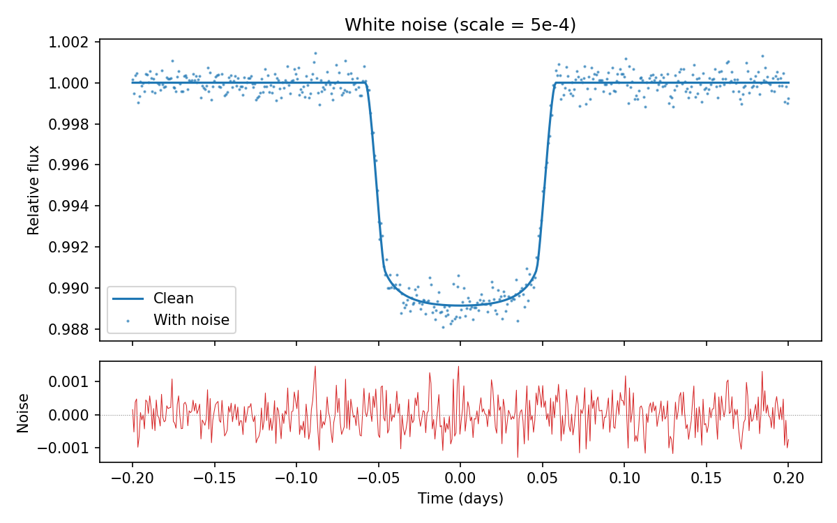
White noise
white_noise() adds independent Gaussian
noise to each flux measurement. The scale parameter controls the
standard deviation:
data = light_curves(
    time=time,
    system=system_strategy,
    noise=st.just(white_noise(scale=5e-4)),
).example()

# data.flux           — clean transit
# data.flux_with_noise — transit + noise
# data.noise           — the noise realisation alone
import numpy as np
import matplotlib.pyplot as plt
from hypothesis import strategies as st
from lightcurve_strategies import (
    bodies, centrals, surfaces, surface_systems,
    light_curves, white_noise,
)

time = np.linspace(-0.2, 0.2, 500)
system_strategy = surface_systems(
    central=centrals(mass=st.just(1.0), radius=st.just(1.0)),
    central_surface=surfaces(u=st.just((0.1, 0.3))),
    body=st.tuples(
        bodies(period=st.just(3.0), radius=st.just(0.1),
               time_transit=st.just(0.0), impact_param=st.just(0.3)),
        surfaces(),
    ),
    min_bodies=1, max_bodies=1,
)

data = light_curves(
    time=time,
    system=system_strategy,
    noise=st.just(white_noise(scale=5e-4)),
    seed=st.just(42),
).example()

fig, (ax1, ax2) = plt.subplots(2, 1, figsize=(8, 5), sharex=True,
                                gridspec_kw={"height_ratios": [3, 1]})
ax1.plot(time, data.flux, label="Clean", linewidth=1.5)
ax1.scatter(time, data.flux_with_noise, s=1, alpha=0.6, label="With noise")
ax1.set_ylabel("Relative flux")
ax1.set_title("White noise (scale = 5e-4)")
ax1.legend()

ax2.plot(time, data.noise, color="tab:red", linewidth=0.5)
ax2.set_xlabel("Time (days)")
ax2.set_ylabel("Noise")
ax2.axhline(0, color="gray", linewidth=0.5, linestyle=":")
fig.tight_layout()
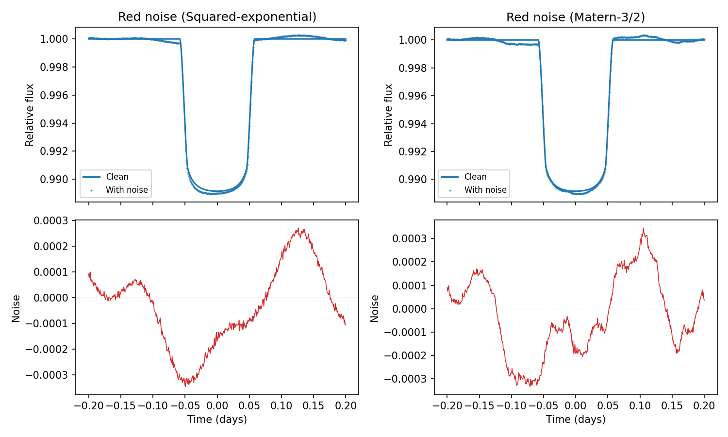
Red noise (correlated)
Real photometric data often exhibits time-correlated (“red”) noise
from stellar variability or instrumental systematics.
red_noise() generates correlated noise
via Cholesky decomposition of a covariance matrix built from a kernel
function.
Two kernels are provided:
sq_exp_kernel()— squared-exponential (RBF): smooth, infinitely differentiable correlations.matern32_kernel()— Matern-3/2: rougher, more realistic stellar variability.
# Squared-exponential red noise
noise_fn = red_noise(
    kernel=sq_exp_kernel(amplitude=3e-4, length_scale=0.05),
    jitter=1e-10,
)

data = light_curves(
    time=time,
    system=system_strategy,
    noise=st.just(noise_fn),
).example()
import numpy as np
import matplotlib.pyplot as plt
from hypothesis import strategies as st
from lightcurve_strategies import (
    bodies, centrals, surfaces, surface_systems,
    light_curves, red_noise, sq_exp_kernel, matern32_kernel,
)

time = np.linspace(-0.2, 0.2, 500)
system_strategy = surface_systems(
    central=centrals(mass=st.just(1.0), radius=st.just(1.0)),
    central_surface=surfaces(u=st.just((0.1, 0.3))),
    body=st.tuples(
        bodies(period=st.just(3.0), radius=st.just(0.1),
               time_transit=st.just(0.0), impact_param=st.just(0.3)),
        surfaces(),
    ),
    min_bodies=1, max_bodies=1,
)

fig, axes = plt.subplots(2, 2, figsize=(10, 6), sharex=True)

for col, (kernel_fn, kernel_name) in enumerate([
    (sq_exp_kernel(amplitude=3e-4, length_scale=0.05), "Squared-exponential"),
    (matern32_kernel(amplitude=3e-4, length_scale=0.05), "Matern-3/2"),
]):
    data = light_curves(
        time=time,
        system=system_strategy,
        noise=st.just(red_noise(kernel=kernel_fn, jitter=1e-10)),
        seed=st.just(42),
    ).example()

    axes[0, col].plot(time, data.flux, label="Clean", linewidth=1.5)
    axes[0, col].scatter(time, data.flux_with_noise, s=1, alpha=0.6,
                         label="With noise")
    axes[0, col].set_ylabel("Relative flux")
    axes[0, col].set_title(f"Red noise ({kernel_name})")
    axes[0, col].legend(fontsize=8)

    axes[1, col].plot(time, data.noise, color="tab:red", linewidth=0.8)
    axes[1, col].set_xlabel("Time (days)")
    axes[1, col].set_ylabel("Noise")
    axes[1, col].axhline(0, color="gray", linewidth=0.5, linestyle=":")

fig.tight_layout()
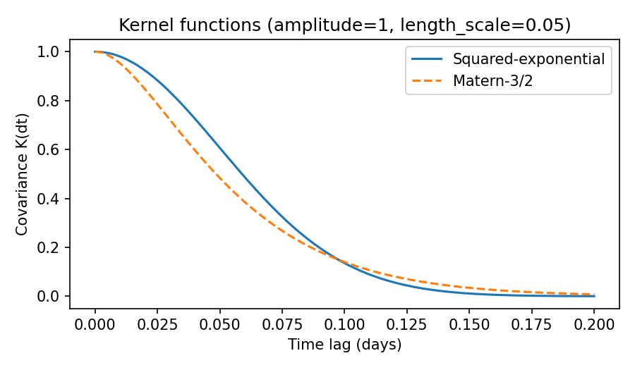
Kernel comparison
The two kernels differ in smoothness. This plot shows the covariance as a function of time lag for both kernels with the same amplitude and length scale:
import numpy as np
import matplotlib.pyplot as plt
from lightcurve_strategies import sq_exp_kernel, matern32_kernel

dt = np.linspace(0, 0.2, 200)
k_se = sq_exp_kernel(amplitude=1.0, length_scale=0.05)
k_m32 = matern32_kernel(amplitude=1.0, length_scale=0.05)

fig, ax = plt.subplots(figsize=(6, 3.5))
ax.plot(dt, k_se(dt), label="Squared-exponential", linewidth=1.5)
ax.plot(dt, k_m32(dt), label="Matern-3/2", linewidth=1.5, linestyle="--")
ax.set_xlabel("Time lag (days)")
ax.set_ylabel("Covariance K(dt)")
ax.set_title("Kernel functions (amplitude=1, length_scale=0.05)")
ax.legend()
fig.tight_layout()
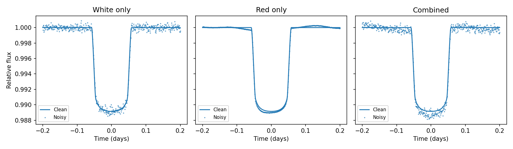
Combined noise
combined_noise() sums multiple noise
sources. This is useful for modelling, e.g., white photon noise on
top of correlated stellar variability:
noise_fn = combined_noise(
    white_noise(scale=3e-4),
    red_noise(kernel=sq_exp_kernel(amplitude=3e-4, length_scale=0.05),
              jitter=1e-10),
)

data = light_curves(
    time=time,
    system=system_strategy,
    noise=st.just(noise_fn),
).example()
import numpy as np
import matplotlib.pyplot as plt
from hypothesis import strategies as st
from lightcurve_strategies import (
    bodies, centrals, surfaces, surface_systems,
    light_curves, white_noise, red_noise, combined_noise, sq_exp_kernel,
)

time = np.linspace(-0.2, 0.2, 500)
system_strategy = surface_systems(
    central=centrals(mass=st.just(1.0), radius=st.just(1.0)),
    central_surface=surfaces(u=st.just((0.1, 0.3))),
    body=st.tuples(
        bodies(period=st.just(3.0), radius=st.just(0.1),
               time_transit=st.just(0.0), impact_param=st.just(0.3)),
        surfaces(),
    ),
    min_bodies=1, max_bodies=1,
)

fig, axes = plt.subplots(1, 3, figsize=(12, 3.5), sharey=True)

configs = [
    ("White only", white_noise(scale=3e-4)),
    ("Red only", red_noise(kernel=sq_exp_kernel(3e-4, 0.05), jitter=1e-10)),
    ("Combined", combined_noise(
        white_noise(scale=3e-4),
        red_noise(kernel=sq_exp_kernel(3e-4, 0.05), jitter=1e-10),
    )),
]

for ax, (title, noise_fn) in zip(axes, configs):
    data = light_curves(
        time=time,
        system=system_strategy,
        noise=st.just(noise_fn),
        seed=st.just(42),
    ).example()
    ax.plot(time, data.flux, linewidth=1.5, label="Clean")
    ax.scatter(time, data.flux_with_noise, s=1, alpha=0.6, label="Noisy")
    ax.set_title(title)
    ax.set_xlabel("Time (days)")
    ax.legend(fontsize=8)

axes[0].set_ylabel("Relative flux")
fig.tight_layout()
Deterministic seeds
Noise is fully reproducible when you fix the seed parameter.
This is useful for regression tests — the same seed always produces
the same noise realisation:
strategy = light_curves(
    time=time,
    system=system_strategy,
    noise=st.just(white_noise(scale=1e-3)),
    seed=st.just(12345),
)

data1 = strategy.example()
data2 = strategy.example()
assert np.array_equal(data1.noise, data2.noise)  # always True
When seed is left as the default (st.integers(0, 2**32 - 1)),
Hypothesis controls the seed, providing determinism within each test
run and shrinkability on failure.
Property-based test with noise
Here is a property-based test that asserts a physical invariant: even with noise added, the clean flux should never exceed the out-of-transit baseline. The noise realisation is checked separately:
from hypothesis import given, settings

@given(
    data=light_curves(
        time=time,
        system=system_strategy,
        noise=st.just(white_noise(scale=1e-3)),
    )
)
@settings(max_examples=10)
def test_clean_flux_bounded(data):
    baseline = data.flux[0]
    assert np.all(data.flux <= baseline + 1e-6)

    # Verify noise was applied correctly
    np.testing.assert_allclose(
        data.flux_with_noise, data.flux + data.noise
    )